Introduction
Background
The primary motivation behind recommendation systems is to help users discover new and relevant items or content that they may be interested in. These systems leverage user data and historical behavior to provide personalized recommendations, which can lead to increased engagement, satisfaction, and retention.
Another key motivation behind recommendation systems is to improve business outcomes for companies. By improving user engagement, satisfaction, and retention, recommendation systems can lead to increased revenue, customer loyalty, and brand advocacy. Additionally, these systems can help companies optimize their product offerings and marketing strategies by providing insights into user preferences and behavior.
Understand the data matrix of user’s ratings
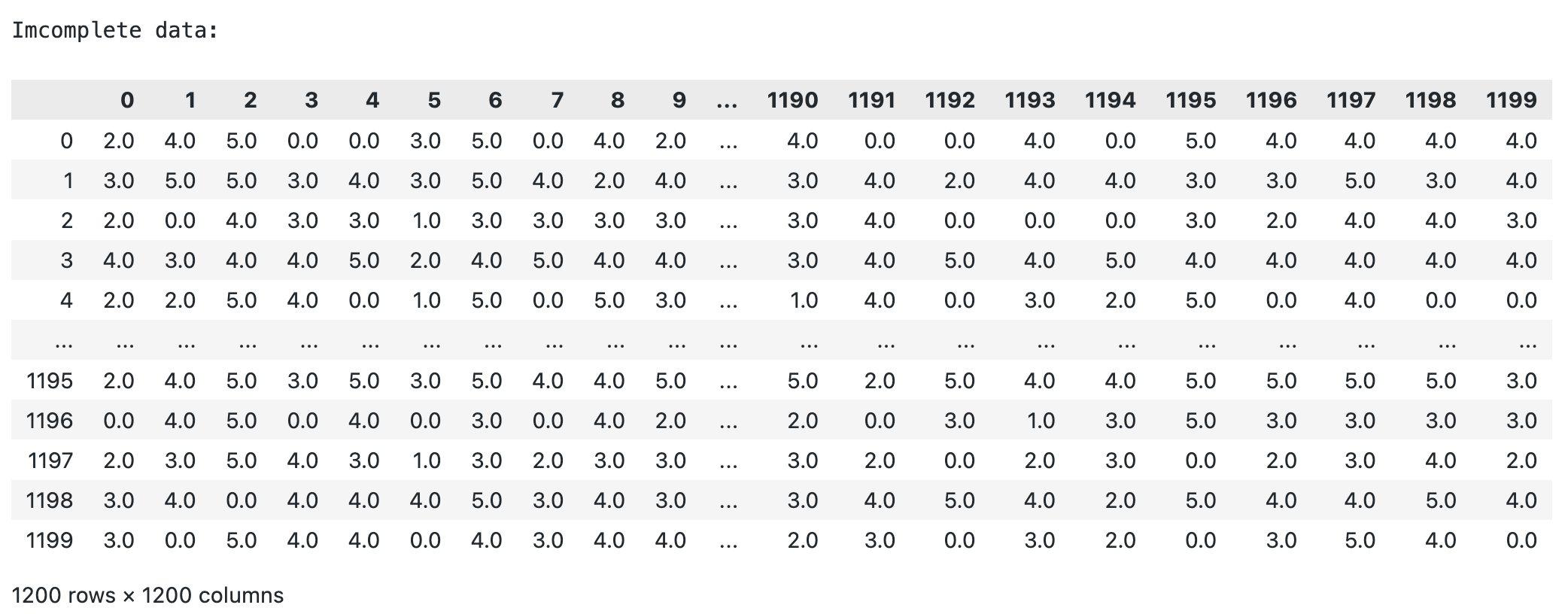
Let X denote the (n,d) data matrix. The rows of this matrix correspond to users and columns specify movies so that X[u,i] gives the rating value of user u for movie i (if available). Both n and d are usually quite large. The ratings range from one to five stars and are mapped to integers {1,2,3,4,5}. We will set X[u,i] = 0 whenever the entry is missing.
Methodology
Normal or Gaussian Distribution
In real life, many datasets can be modeled by Gaussian Distribution (Univariate or Multivariate). So it is quite natural and intuitive to assume that the clusters come from different Gaussian Distributions. Or in other words, it tried to model the dataset as a mixture of several Gaussian Distributions. This is the core idea of this model. In one dimension the probability density function of a Gaussian Distribution is given by
\[G(X|\mu, \sigma) = \dfrac{1}{\sigma \sqrt{2\pi}} e^{\dfrac{-(x - \mu)}{2\sigma^2}}\]where $\mu$ and $\sigma^2$ are respectively the mean and variance of the distribution. For multivariate (let us say d-variate) Gaussian Distribution, the probability density function is given by
\[G(X|\mu,\sum) = {1\over \sqrt{(2\pi)|\sum|}} exp(-{1\over 2} {(X-\mu)}^T{\textstyle \sum^{-1}}(X-\mu))\]Here $\mu$ is a d-dimensional vector denoting the mean of the distribution and $\sum$ is the d*d covariance matrix
Gaussian Mixture Model
Suppose there are K clusters (For the sake of simplicity here it is assumed that the number of clusters is known and it is K). So $\mu$ and $\sum$ are also estimated for each k. Had it been only one distribution, they would have been estimated by the maximum-likelihood method. But since there are K such clusters and the probability density is defined as a linear function of densities of all these K distributions, i.e.
\[p(X) = \sum_{k=1}^K \pi_kG(X|\mu_k,{\textstyle\sum_k})\]where $\pi_k$ is the mixing coefficient for $k^{th}$ distribution.
Mixture model for Matrix Completion
We can now extend our Gaussian mixture model to predict actual movie ratings. Remember how we set up X (n,d) matrix as our data matrix. In realistic setting, most of the entries of X are missing. For this reason, we define $C_u$ as a set of movies (column indexes) that user u has rated and $H_u$ as its complement (the set of remaining unrated movies we wish to predict ratings for). We use $|C_u|$ to denote the number of observed rating values from user u. From our mixture model, each user u is an example $x^{(u)} = X[u,:]$. But since most of the coordinates of $x^{(u)}$ we need to focus the model during training on just the observed entries. To this end, we use $x_{C_u}^{(u)}$ = { $x_i^{(u)} : i\in C_u$ } as the vector of only observed ratings. If columns are indexed as { 0,1,…,d-1}, then a user u with a rating vector $x^{(u)}$ = {5,4,0,0,2}, where zeros indicates missing values, has $C_u$ = {0,1,4}. $H_u$ = {2,3}, and $x_{C_u}^{(u)} = (5,4,2)$
In this part, we will extend our mixture model in two key ways
- First, we are going to estimate a mixture model based on partially observed ratings.
- Second, since we will be dealing with a large, high-dimensional data set, we will need to be more careful of numerical underflow issues. We should use the “log trick” to avoid the situation. Remember log(a*b) = log(a) + log(b). This can be useful to remember when a and b are very small, in this case, addition should result in fewer numerical underflow issues than multiplication.
Marginalizing over unobserved coordinates
First, we introduce the notation:
- X: an (n,d) Numpy array of n data points, each with d features ( n users with d movies )
- K: number of mixtures components
- $\mu$: (K,d) Numpy array where the $j^{th}$ row is the mean vector $\mu^{(j)}$
- p: (K,) Numpy array of mixing proportions $\pi_j$,j=1,…,K
- var: (K,) Numpy array of variances $\sigma_j^2$,j=1,2,…,K
If $x^{(u)}$ were a complete rating vector, the mixture model would simply say that
\[P(x^{(u)} | \theta) = \sum_{j=1}^K \pi_jN(x^{(u)};\mu^{(u)},\sigma_j^2I)\]In the presence of missing values, we must use the marginal probability $ P(x_{C_u}^{(u)} \theta) $ that is over only the observed values.
This marginal corresponds to integrating the mixture density $P(x^{(u)} | \theta)$ over all the unobserved coordinate values. In our case, this marginal can be computed as follows.
The mixture model for a complete rating vector is written as:
\[P(x^{(u)}|\theta) = \sum_{j=1}^K p_jN(x^{(u)};\mu^{(j)},\sigma_j^2I)\]Because the multivariate Gaussian as a product of univariate Gaussians (since there is no covariance between coordinates)
\[P(x^{(u)}|\theta) = \sum_{j=1}^Kp_j\prod_i N(x_i^{(u)};\mu_i^{(j)},\sigma_i^{2,(j)})\] \[= \sum_{j=1}^Kp_j\prod_{m \in C_u} N(x_m^{(u)};\mu_m^{(j)},\sigma_m^{2,(j)}) \prod_{m' \in H_u} N(x_{m'}^{(u)};\mu_{m'}^{(j)},\sigma_{m'}^{2,(j)})\]For $m’ \in H_u$, we can marginalize over all of the unobserved values to get
\[\int N(x_{m'}^{(u)};\mu_{m'}^{(j)},\sigma_{m'}^{2,(j)})dx_{m'}^{(u)} = 1\]Then, our mixture density can be written as
\[P(x_{C_u}^{(u)}|\theta) = \sum_{j=1}^Kp_jN(x_{C_u}^{(u)};\mu_(C_u)^{(j)},\sigma_j^2I_{|C_u|*|C_u|})\]where $I_{|C_u|*|C_u|}$ is the identity matrix in $|C_u|$ dimensionss
Expectation-Maximization (EM) algorithm
The Expectation-Maximization (EM) algorithm is an iterative way to find maximum-likelihood estimates for model parameters when the data is incomplete or has some missing data points or has some hidden variables. EM chooses some random values for the missing data points and estimates a new set of data. These new values are then recursively used to estimate a better first date, by filling up missing points, until the values get fixed.
In the Expectation-Maximization (EM) algorithm, the estimation step (E-step) and maximization step (M-step) are the two most important steps that are iteratively performed to update the model parameters until the model convergence.
The E-step update is:
\[p(j|t) = { {p_jN(x;\mu^{(j)},\sigma_j^2I)} \over \sum_{j=1}^K p_j N(x;\mu^{(j)},\sigma_j^2I)}\]The M-step update is:
\[\hat{n}_j = \sum_{t=1}^n p(j|t)\] \[\hat{p}_j = {\hat{n}_j\over n}\] \[\hat{\mu^{(j)}} = {1\over{\hat{n}_j}}\sum_{t=1}^n p(j|t)x^{(t)}\] \[\hat{\sigma_j}^2 = {1\over d\hat{n}_j}\sum_{t=1}^n p(j|t)||x^{(t)} - \hat{\mu}^{(j)}||^2 \]EM algorithm for matrix completion
We need to update our EM algorithm a bit to deal with the fact that the observations are no longer complete vectors. We use Bayes’ rule to find an updated expression for the posterior probability $p(j|u) = P(y=j|x_{C_u}^{(u)})$ :
\[p(j|u) = {p(u|j).p(j)\over p(u)} = {p(u|j).p(j)\over \sum_{j=1}^K p(u|j).p(j)}\] \[= {\pi_jN(x_{C_u}^{(u)};\mu_{C_u}^{(u)},\sigma_j^2I_{C_u*C_u}) \over \sum_{j=1}^K \pi_jN(x_{C_u}^{(u)};\mu_{C_u}^{(j)},\sigma_j^2I_{|C_u|*|C_u|})}\]Maximizing likelihood function, we get :
\[\hat{\mu_l}^{(k)} = {\sum_{u=1}^n p(k|u)\delta(l,C_u)x_l^{(u)}\over \sum_{u=1}^n p(k|u)\delta(l,C_u) }\]( where $\delta(i,C_u) = 1$ if $i\in C_u$ and $\delta(i,C_u) = 0 $ if $i \notin C_u$ )
\[\hat{\sigma_k}^2 = {1\over\sum_{u=1}^n |C_u|p(k|u)}\sum_{u=1}^np(k|u)||x_{C_u}^{(u)}-\hat{\mu}_{C_u}^{(k)}||^2\] \[\hat{\pi_k} = {1\over n}\sum_{u=1}^n p(k|u)\]Completing missing entries
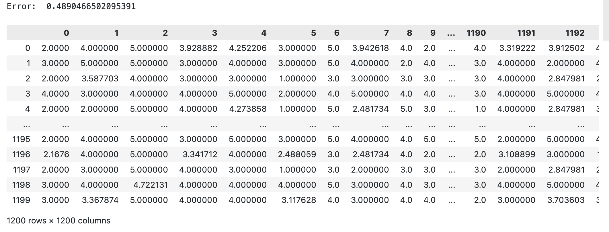
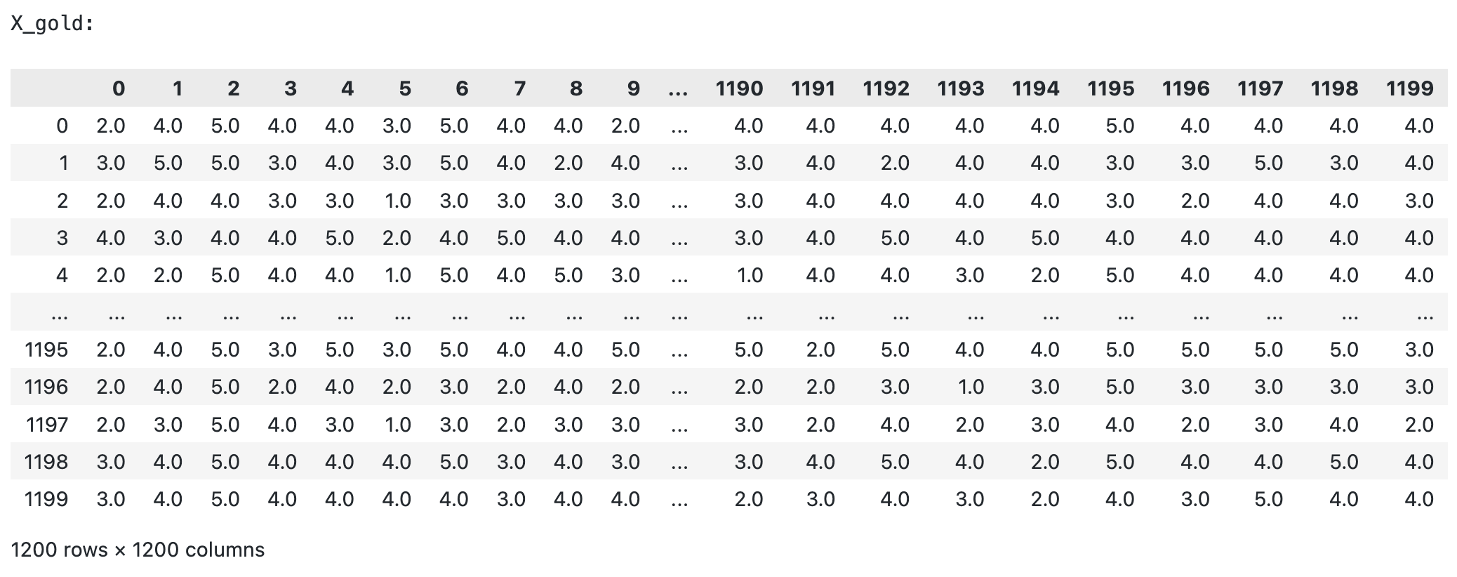
To complete the row $x_i^{(u)}$ for all values of $ i \notin C$ where C is the set of observed values, we have:
\[x_i^{(u)} = \sum_{j=1}^k p(j|u)\mu_i^{(j)}\]Experiments
Data set: Netflix movie ratings data set (1200 * 1200)
Tuning the hyperparameter K ( the number of Gaussians in our Gaussian mixture model) in range of (10,15). We got the best K is 10 with error of 0.489