Bayesian Statistics (MIT)

17. Bayesian Statistics

18. Bayesian Statistics (cont.)

Frequentist approach:

• Observe data
• These data were generated randomly (by nature, by measurement, by designing a survey, etc…)
• We made assumptions on the generating process e.g., i.i.d., Gaussian data, smooth density, linear regression function, etc…)
• The generating process was associated to some object of interest (e.g., a parameter, a density, etc…)
• This object was unknown but fixed and we wanted to find it: we either estimated it or tested a hypothesis about this object, etc…

Bayesian approach:

• We still observe data, assumed to be randomly generated by some process. Under some assumptions (e.g., parametric distribution), this process is associated with some fixed object.
• We have a prior belief about it

• Using the data, we want to update that belief and transform it into a posterior belief

• Example:
  • Let p be the proportion of woman
  • Sample n people randomly with replacement in the population and denote by $X_i \overset{\mathrm{iid}}{\sim}$ Bern(p)
  • In the frequentist approach, we estimated p (using MLE), we constructed some confidence interval for p, we did hypothesis testing
  • Before analyzing data, we may believe that p is likely close to $1\over 2$
  • Bayesian approach is a tool to :
    • include mathematically our prior belief in statistical procedures
    • update our prior belief using the data
  • Our prior belief about p can be quantified:
    • E.g., we are 90% sure that p is between .4 and .6, 95% that it is between .3 and .8, etc…

  ⇒ We can model our prior belief using a distribution for p, as if p was random

• In reality, the true parameter is not random ! However, the Bayesian approach is a way of modeling our belief about the parameter by doing as if it was random.
  • e.g: $p \sim B(a,a)$ (Beta distribution) for some a>0

  → This distribution is called prior distribution

  • In our statistical experiment, $X_1,…,X_n$ are assumed to be i.i.d. Bernoulli with parameter p conditionally on p.
  • After observing the available sample $X_1,…,X_n$ we can update our belief about p by taking its distribution conditionally on the data
  • The distribution of p conditionally on the data is called posterior distribution

Conjugate probability:

• Refer to a situation in Bayesian statistic where the prior and the the posterior belong to the same family of probability distributions.
• For example, if we assume that the prior of a parameter is a normal distribution, and we observe some date, then the posterior of that parameter will also be a normal distribution. In this case, we say that the normal distribution is a conjugate prior for the parameter.
• The advantage is that it allows for the analytical calculation of the posterior distribution, which can simplify the Bayesian inference process. Additionally, using a conjugate prior distribution can provide intuitive interpretation of the posterior distribution, and can also help to reduce the computational burden of Bayesian inference.
• Bayesian inference :
  • Bayesian inference is a statistical approach for updating the probability of a hypothesis or parameter based on new evidence or data. In Bayesian inference, the prior probability distribution represents the initial belief or knowledge about the hypothesis or parameter, and the posterior probability distribution represents the updated belief or knowledge about the hypothesis or parameter after considering the new evidence or data.

  The basic steps in Bayesian inference are as follows:

  1. Specify a prior probability distribution for the hypothesis or parameter based on previous knowledge or beliefs.
  2. Collect new data or evidence.
  3. Use Bayes’ theorem to update the prior probability distribution to obtain the posterior probability distribution.
  4. Interpret the posterior probability distribution and make decisions or draw conclusions based on it.

  Bayes’ theorem states that the posterior probability distribution is proportional to the product of the prior probability distribution and the likelihood function, which describes the probability of observing the data given the hypothesis or parameter. The normalization constant in Bayes’ theorem ensures that the posterior probability distribution integrates to 1.

  Bayesian inference has several advantages over other statistical approaches. For example, Bayesian inference allows for the incorporation of prior knowledge or beliefs, which can improve the accuracy of statistical inference, especially in situations where the sample size is small. Bayesian inference also provides a flexible framework for modeling complex data structures and can handle missing data and other types of uncertainties. However, Bayesian inference can be computationally intensive, and the choice of prior distribution can have a significant impact on the posterior distribution.

The Bayes rule and posterior distribution:

• Consider a probability distribution on a parameter space $\Theta$ with some pdf $\pi(.)$: the prior distribution
• Let $X_1,…,X_n$ be a sample of n random variables
• Denote by $p_n$: the joint pdf of $X_1,…,X_n$ conditionally on $\theta,$ where $\theta \sim \pi$ (a.k.a likelihood)
• We usually assume that $X_1,…,X_n$ are i.i.d conditionally on $\theta$.
• The conditional distribution of $\theta$ given $X_1,…,X_n$ is called the posterior distribution. Denote by $\pi(.|X_1,…,X_n)$
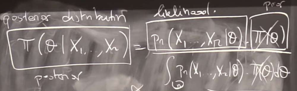
• Bayes’s formula states that:
  • $\pi(\theta|X_1,…,X_n) \propto \pi(\theta)p_n(X_1,…,X_n|\theta)\forall \theta \in \Theta$
• The constant does not depend on $\theta$:
  • $\pi(\theta|X_1,…,X_n) = {\pi(\theta)p_n(X_1,…,X_n|\theta)\over \int_{\Theta}p_n(X_1,…,X_n|t)d_{\pi}(t)} \forall \theta \in \Theta$

Non-informative priors:

• Idea:
  • In case of ignorance, or lack of prior information, one may want to use a prior that is as little informative as possible
• Good candidate: $\pi(\theta) \propto 1$, i.e., constant pdf on $\Theta$.
  • If $\Theta$ is bounded, this is uniform prior on $\Theta$.
  • If $\Theta$ is unbounded, this does not define a proper pdf on $\Theta$.
• An improper prior on $\Theta$ is a measurable, non-negative function $\pi(.)$ defined on $\Theta$ that is not integrable.

• In general, we can still define a posterior distribution using an improper prior, using Bayes’s formula.

  

• Example:

  • If $p \sim U(0,1)$ and given $p,X_1,\cdots,X_n \stackrel{\text{i.i.d.}}{\sim} Ber(p):$

    

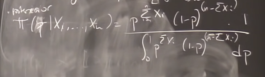
    $\pi(p|X_1,\cdots,X_n)\propto p^{\sum_{i=1}^n X_i} (1-p)^{n-\sum_{i=1}^n X_i}$

    ⇒ the posterior distribution is:

    $B(1+\sum_{i=1}^nX_i,1+n-\sum_{i=1}^nX_i)$

  • If $\pi(\theta) = 1 \forall \theta \in R$ and given $\theta, X_1,…,X_n \stackrel{\text{i.i.d.}}{\sim} N(\theta,1)$ :

    $\pi(\theta|X_1,…,X_n) \propto \exp(-{1\over 2}\sum_{i=1}^n(X_i-\theta)^2)$

    ⇒ The posterior distribution is:

    \[N(\bar X_n,{1\over n})\]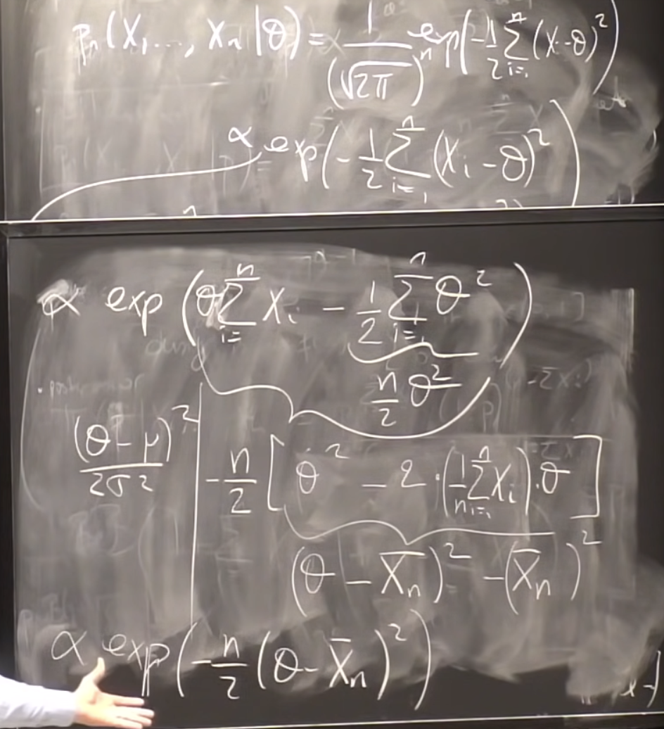

    

• Jeffreys prior :
  • $\pi_J(\theta) \propto \sqrt{\det I(\theta)}$ where $I(\theta)$ is the Fisher information matrix of the statistical model associated with $X_1,…,X_n$ in the frequentist approach (provided if exists)
  • Jeffreys prior satisfies a re-parametrization invariance principle:

    • If $\eta$ is a re-parametrization of $\theta$(i.e., $\eta = \phi(\theta)$ for some one-to-one map $\phi$), then the pdf $\widetilde{\pi}(.)$ of $\eta$ satisfies: $\widetilde{\pi}(\eta)\propto \sqrt{\det \widetilde{I}(\eta)}$,

      Where $\widetilde{I}(\eta)$ is the Fisher information of the statistical model parametrized by $\eta$ instead of $\theta$.

Bayesian confidence region

• For $\alpha \in (0,1)$, a Bayesian confidence region with level $\alpha$ is a random subset R of the parameter space $\Theta$, which depends on the sample $X_1,…,X_n$ such that:
  • $P[\theta \in R | X_1,…,X_n] = 1-\alpha$
  • Note that R depends on the prior $\pi(.)$
• Bayesian confidence region and confidence interval are two distinct notions.
• Example:
  • $X_1 = \theta +\epsilon_1,X_2= \theta+\epsilon_2$ where $P(\epsilon_i=1)=P(\epsilon_i=-1)={1\over2}$
  • $R=\begin{cases} X_1-1 ,if X_1=X_2 \over {X_1+X_2\over 2},if X_1 ≠ X_2\end{cases}$

  ⇒ This is confidence region (Frequentist) at level 75%

• Bayes region: $P(\theta \in {X_1-1} \cap X_1≠X_2) + P(\theta\in {X_1+X_2\over2} \cap X_1≠X_2)$ = $P(\theta=\theta+\epsilon_1-\epsilon_2\cap\epsilon_1=\epsilon_2) +P(\epsilon_1+\epsilon_2 = 0\cap \epsilon_1≠\epsilon_2)$ = 1/4 + 2/4 = 3/4

• Likelihood: $P(X_1,X_2|\theta)$

  Let assume that $X_1=5,X_2=7$.

  $P(5,7|\theta) = \begin{cases} 1/4,if \theta=6\over 0, otherwise \end{cases}$

  posterior: $\pi(\theta|5,7) = {\pi(\theta)p(5,7|\theta)\over \sum_{t\in Z}\pi(t)p(5,7|t)}$

  ⇒ $\pi(\theta|5,7) = \begin{cases} 1,if \theta=6 \over 0, otherwise \end{cases}$

• Bayesian estimation:
  • The Bayes framework can be used to estimate the true underlying parameter
  • In this case, the prior does not reflect a prior belief: It is just an artificial tool used in order to define a new class of estimators.
  • Define a distribution (that can be improper) with pdf $\pi$ on the parameter space $\Theta$.
  • Compute the posterior pdf $\pi(.|X_1,…,X_n)$ associated with $\pi$, seen as a prior distribution
  • Bayes estimator:
  \[\hat\theta^{(\pi)} = \int_{\Theta}\theta d_{\pi}(\theta|X_1,...,X_n)\]

  This is the posterior mean.

  • The Bayesian estimator depends on the choice of the prior distribution $\pi$
  • In general, the asymptotic properties of the Bayes estimator do not depend on the choice of the prior.