Neural Machine Translation with RNN attention model

code

In Machine Translation, the goal is to convert a sentence from the source language to the target language. We will describe the training procedure for the NMT system, which uses a Bidirectional LSTM Encoder and Unidirectional LSTM Decoder.

Given a sentence in the source language, we look up the word embeddings from an embeddings matrix, yielding $x_1,x_2,…,x_m|x_i \in R^e$ where m is the length of the source sentence and e is the embedding size. We feed these embeddings to the bidirectional Encoder, yielding hidden states and cell states for both forwards (→) and backwards (←) LSTMs. The forwards and backwards versions are concatenated to give hidden states $h_i^{enc}$ and cell states $c_i^{enc}$:

\[h_i^{enc} = [\overleftarrow {h_i^{enc}} ; \overrightarrow{h_i^{enc}}]\] \[c_i^{enc} = [\overleftarrow{c_i^{enc}};\overrightarrow{c_i^{enc}}]\]

where $h_i^{enc} \in R^{2h} , \overleftarrow{h_i^{enc}},\overrightarrow{h_i^{enc}} \in R^{h} \forall 1 ≤ i≤ m$ and $c_i^{enc} \in R^{2h}, \overleftarrow{c_i^{enc}},\overrightarrow{c_i^{enc}} \in R^{h} \forall 1≤i≤m$

We then initialize the Decoder’s first hidden state $h_0^{dec}$$h_o^{dec}$ and cell state $c_0^{dec}$ with a linear projection of the Encoder’s final hidden state and final cell state.

\[h_0^{dec} = W_h[\overleftarrow{h_1^{enc}};\overrightarrow {h_m^{enc}}]\] \[c_0^{dec} = W_c[\overleftarrow{c_1^{enc}};\overrightarrow{c_m^{enc}}]\]

where $h_0^{dec},c_0^{dec} \in R^{h.1}$ and $W_h,W_c \in R^{h.2h}.$

With the Decoder initialized, we must now feed it to a matching sentence in the target language. On $t^{th}$ step, we look up the embedding for the $t^{th}$ word, $y_t \in R^{e}$. We then concatenate $y_t$ with combined-output vector $o_{t-1} \in R^{h}$ from the previous time-step to produce $\bar {y_t} \in R^{(e+h)}$. Note that for the first target word (i.e. the start token) $o_0$ is a zero-vector. We then feed $\bar{y_t}$ as input to the Decoder LSTM

\[h_t^{dec},c_t^{dec} = Decoder(\bar{y_t},h_{t-1}^{dec},c_{t-1}^{dec})\]

where $h_t^{dec}\in R^{h} ,c_t^{dec} ]\in R^{h}$.

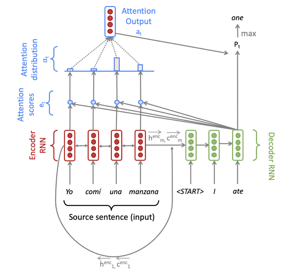
We then use $h_t^{dec}$ to compute multiplicative attention over $h_0^{enc},…,h_m^{enc}:$

\[e_{t,i}= (h_t^{dec})^TW_{attProj}h_i^{enc}\] \[\alpha_t = Softmax(e_t)\] \[a_t = \sum_i^m \alpha_{t,i} h_i^{enc}\]

where $e_t,\alpha_t \in R^{m}, W_{attProj}\in R^{h.2h} , a_t \in R^{2h}$.

We now concatenate the attention output $a_t$ with the decoder hidden state $h_t^{dec}$ and pass this through a linear layer, Tanh, and Dropout to attain the combined-output vector $o_t$.

\[u_t = [a_t;h_t^{dec}]\] \[v_t = W_uu_t\] \[o_t=Dropout(Tanh(v_t))\]

where $o_t,v_t \in R^{h};u_t \in R^{3h} ; W_u \in R^{h.3h}$

Then we produce a probability distribution P, over target words at the $t^{th}$ time-step:

\[P_t = Softmax(W_{vocab}o_t)\]

where $P_t \in R^{V_t1} , W_{vocab}\in R^{V_t.h}$.

Here, $V_t$ is the size of the target vocabulary. Finally, to train the network we then compute the softmax cross entropy loss between $P_i$ and $g_t$, where $g_t$ is the one-hot vector of the target word at time-step t:

\[J_t(\theta) = CE(P_t,g_t)\]

Here, $\theta$ represents all the parameters of the model and $J_t(\theta)$ is the loss on step t of the decoder.

---