Home World Game RL project

tranquocde/MITx_686x/tree/main/rl

Description

In this project, we will consider a text-based game represented by the tuple $<H,C,P,R,\gamma ,\Psi >$ . Here H is the set of all possible game states. The actions taken by the player are multi-word natural language commands such as eat apple or go east . In this project we limit ourselves to consider commands consisting of one action (e.g., eat ) and one argument object (e.g. apple ).

• H : set of all possible game states. (room , quest)
• $C={ (a,b)}$ is the set of all commands (action-object pairs)
• $P:H\times C\times H\rightarrow [0,1]$ is the transition matrix $P(h’|h,a,b)$ is the probability of reaching state h’ if command c = (a,b) is taken in state h.
• $R:H\times C\rightarrow \mathbb {R}$ is the deterministic reward function: $R(h,a,b)$ is the immediate reward player contains when taking command (a,b) in state h.
• Discounted factor $\gamma$

The game state h is hidden from the player , who only receives a varying textual description.

• S denotes the space of all possible text descriptions. The text description $s$ observed by the player are produced by a stochastic function $\Psi :H\rightarrow S$ . Assume that each observable state $s \in S$ is associated with a unique hidden state, denoted by $h(s) \in H$.

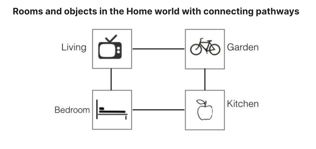
You will conduct experiments on a small Home World, which mimic the environment of a typical house. The world consists of four rooms- a living room, a bed room, a kitchen and a garden with connecting pathways (illustrated in figure below). Transitions between the rooms are deterministic. Each room contains a representative object that the player can interact with. For instance, the living room has a TV that the player can watch , and the kitchen has an apple that the player can eat. Each room has several descriptions, invoked randomly on each visit by the player.

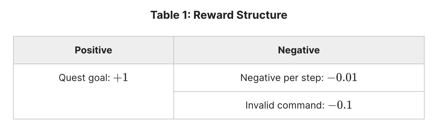
At the beginning of each episode, the player is placed at a random room and provided with a randomly selected quest. An example of a quest given to the player in text is You are hungry now. To complete this quest, the player has to navigate through the house to reach the kitchen and eat the apple (i.e., type in command eat apple). In this game, the room is hidden from the player, who only receives a description of the underlying room. The underlying game state is given by $h=(r,q)$ , where $r$ is the index of room and $q$ is the index of quest. At each step , the text description s is provided to the player contains 2 parts $s=(s_r , s_q)$ where $s_r$ is the room description (varied and randomly provided) and $s_q$ is quest description. The player receives a positive reward on completing a quest, and negative rewards for invalid command (e.g., eat TV). Each non-terminating step incurs a small deterministic negative rewards, which incentives the player to learn policies that solve quests in fewer steps. (see the Table 1) An episode ends when the player finishes the quest or has taken more steps than a fixed maximum number of steps.

Each episode produces a full record of interaction $(h_{0},s_{0},a_{0},b_{0},r_{0},… ,h_{t},s_{t},a_{t},b_{t},r_{t},h_{t+1}… )$

where $h_{0}=(h_{r,0},h_{q,0})\sim \Gamma _{0}$ ($\Gamma _{0}$ denotes an initial state distribution)

$h_{t}\sim P(\cdot |h_{t-1},a_{t-1},b_{t-1})$ , $s_{t}\sim \Psi (h_{t})$ , $r_t=R(h_t,a_t,b_t)$ and all commands $(a_t,b_t)$ are chosen by the player.

The record of interaction observed by the player is $(s_{0},a_{0},b_{0},r_{0},\ldots ,s_{t},a_{t},b_{t},r_{t},\ldots )$. Within each episode, the quest remains unchanged, i.e., $h_{q,t} = h_{q,0}$ (so as the quest description $s_{q,t} = s_{q,0}$ ).When the player finishes the quest at time $K$ , all rewards after time $K$ are assumed to be zero, i.e., $r_t=0$ for $t>K$ . Over the course of the episode, the total discounted reward obtained by the player is

Note that the hidden state $h_0,…,h_T$ are unobservable to the player.

The learning goal of the player is to find a policy that $\pi:S\rightarrow C$ that maximizes the expected cumulative discounted reward

$\mathbb {E}[\sum_{t=0}^{\infty }\gamma ^{t}R(h_{t},a_{t},b_{t})| (a_{t},b_{t})\sim \pi ],$ where the expectation accounts for all randomness in the model and the player.

Let $\pi^*$ denote the optimal policy. For each observable state , let be the associated hidden state. The optimal expected reward achievable is defined as

where

We can define optimal Q-function as

Note that given $Q^*(s,a,b)$ we can obtain an optimal policy:

• The commands set $C$ contain all (action , object) pairs. Note that some commands are invalid. For instance, (eat,TV) is invalid for any state, and (eat, apple) is valid only when the player is in the kitchen (i.e., $h_r$ corresponds to the index of kitchen). When an invalid command is taken, the system state remains unchanged and a negative reward is incurred. Recall that there are four rooms in this game. Assume that there are four quests in this game, each of which would be finished only if the player takes a particular command in a particular room. For example, the quest “You are sleepy” requires the player navigates through rooms to bedroom (with commands such as go east/west/south/north ) and then take a nap on the bed there. For each room, there is a corresponding quest that can be finished there.
• Note that in this game, the transition between states is deterministic. Since the player is placed at a random room and provided a randomly selected quest at the beginning of each episode, the distribution $\Gamma_0$ of the initial state $h_0$ is uniform over the hidden state space H.

Questions

Relation between value function and Q-function

Optimal episodic reward

Assume that the reward function $R(s,a,b)$ is given in Table 1. At the beginning of each game episode , the player is placed in a random room and provided with a randomlhy selected quest. Let $V^*(h_0)$ be the optimal value function for an initial state $h_0$, i.e ,

Solution

Each state consists of $(s_r,s_q)$ with $s_r$ is the room of player and $s_q$ is the quest.

• If player is in the correct room , then the optimal policy is go straight forward to the item. So the reward is 1
• If the player is in the next room of the correct room , then the optimal policy is going through the next room to the correct room and get the item. The reward is $-0.01 + \gamma * 1 = 0.49$
• if the player is in the room next to the next room of the correct room , the the optimal policy is going through 2 rooms and get the item. The reward is $-0.01 - \gamma * 0.01 + \gamma^2*1 = 0.235$

The probability of first case is 4/16 = 0.25 , second case is 8/16 = 0.5 , third case is 4/16 = 0.25

So $\mathbb{E}[V^{*}(h_{0})]$ = 0.25 * 1 + 0.5 * 0.49 + 0.25 * 0.235 = 0.55375

Q-learning algorithm

• The agent plays an action $c$ at state $s$, getting a reward $R(s,c)$ and observing the next state $s’$
• Update the single Q-value corresponding to each such transition

MITx_686x/agent_tabular_ql.py at main · tranquocde/MITx_686x

Epsilon-greedy exploration

• Epsilon-greedy is a simple exploration-exploitation strategy used in reinforcement learning. In this strategy, an agent chooses either the action that it believes is currently the best (exploitation) or a random action (exploration) with some probability epsilon (ε)

Pseudocode for epsilon-greedy:

if random_number < epsilon:
    // Choose a random action
    action = choose_random_action()
else:
    // Choose the best action based on current estimates
    action = argmax(Q[state, :])

Q-learning with linear function approximation

• Since the state displayed to the agent is described in text, we have to choose a mechanism that maps text descriptions into vector representations. A naive way is to create one unique index for each text description, as we have done in previous part. However, such approach becomes infeasible when the state space becomes huge. To tackle this challenge, we can design some representation generator that does not scale as the original textual state space. In particular, a representation generator $\psi_R(\cdot )$ reads raw text displayed to the agent and converts it to a vector representation $v_{s}=\psi_R(s)$. One approach is to use a bag-of-words representation derived from the text description.
• In large games , it is often impractical to maintain the Q-value for all possible state-action pairs. One solution to this problem is to approximate $Q(s,c)$ using a parametrized function $Q(s,c;\theta)$
  • We consider a linear parametric architecture:
  \[Q(s,c;\theta) = \phi(s,c)^T\theta = \sum_{i=1}^d \theta_i(s,c)\theta_i\]

  where $\theta(s,c)$ is a fixed vector in $R^d$ for state-action pair $(s,c)$ with i-th component given by $\theta_i(s,c)$ and $\theta \in R^d$ is a parameter vector that is shared across state-action pairs. The key challenge here is to design feature vectors $\theta(s,c)$. Note that a given textual state $s$, we first translate it to a vector representation $v_s$ using $\psi _{R}(s)$. So the question here is how to design a mapping function convert $(\psi_R(s),c)$ into a vector representation in $R^d$. Assume that the size of action space is $d_C$, and the dimension of the vector space for the state representation is $d_R$.

Computing $\theta$ update rule : The Q-learning approximation algorithm starts with an initial parameter estimate of $\theta$. As the tabular Q-learning , upon observing a data tuple $(s,c,R(s,c),s’)$, the target value y for the Q-value of (s,c) is defined as the sampled version of the Bellman operator,

Then the parameter $\theta$ is simply updated by taking a gradient step w.r.t to the squared loss.

The negative gradient $g(\theta )=-\frac{\partial }{\partial \theta }L(\theta )= (y-Q(s,c,\theta))\phi(s,c)$

Hence the update rule for $\theta$ is :

where $\theta$ is the learning rate.

• Approximate Q-value using linear estimator: (example code)

MITx_686x/agent_linear.py at main · tranquocde/MITx_686x

• Approximate Q-value using neural network :

MITx_686x/agent_dqn.py at main · tranquocde/MITx_686x