Auto-regressive model

Given a dataset $D$ of n-dimensional datapoints x. We assume $ x\in \{ 0,1 \} ^n. $

Chain rule

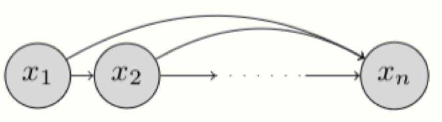
The joint distribution over n-dimensions :

\[p(x) = \prod_{i=1}^n p(x_i|x_1,...,x_{i-1})=\prod_{i=1}^np(x_i|x_{<i})\]

Represent as graphical model :

⇒ How to reproduce the distribution ??? (Given the dataset $D$)

Approach 1: Tabular representation (a.k.a truth table)

Bottleneck : Too much to handle !!!

For example : $p(x_n|x_{<n})$ needs $2^{n-1}$ configurations of previous n-1 variables (because $ x \in \{ 0,1 \}^n$)

⇒ exponential space complexity !!!

Approach 2: Parametrically approximate

\[p_{\theta_i}(x_i|x_{<i})=Bern(f_i(x_1,...,x_{i-1}))\]

where $\theta_i$ denotes the set of params. used to specify the mapping $f_i:{0,1}^{i-1}\rightarrow[0,1]$ ($f_i$ could be a neural network, actually it should be a neural network :D , in a differentiable way !! so we can back-propagate)

⇒ What is the number of params. now ? : $\sum_{i=1}^n | \theta_i |$

For each choice of $f_i$, we get a specific model.

• First, let see the fully-visible sigmoid belief network (FVSBN)

  

  \[f_i(x_1, x_2, \ldots, x_{i-1}) =\sigma(\alpha^{(i)}_0 + \alpha^{(i)}_1 x_1 + \ldots + \alpha^{(i)}_{i-1} x_{i-1})\]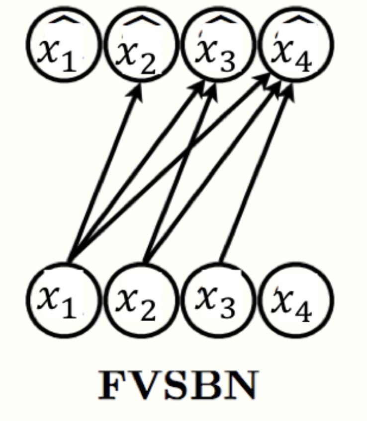

  $\sigma$ denotes the sigmoid function

  $\theta_i = { \alpha_0^{(i)},…,\alpha_{i-1}^{(i)}}$ denote the params. of $f_i(.)$

  ⇒ #num. of params. = $\sum_{i=1}^n i = O(n^2)$

  Much fewer space than tabular approach !!!

• To enhance the expressiveness of an autoregressive model, we can replace $f_i$ by something more flexible parametrize - which is a neural network (or MLP: multilayer perceptron). For example:

  \[h_i = \sigma(A_ix_{<i}+c_i)\] \[f_i(x_1,...,x_{i-1}) = \sigma(\alpha^{(i)}h_i+b_i)\]

  $h_i\in R^d$ : hidden layer activations for the MLP

  $\theta_i={A_i\in R^{d*(i-1)},c_i\in R^d,\alpha^{(i)}\in R^d,b_i \in R}$ : set of params. for the function $f_i(.)$

  #num. of params = $O(n^2d)$

  Still much fewer than tabular approach !!!

  More expressiveness than FVSBN !! ⇒ better accuracy

• Want to reduce #num. of params. of the above model ???

  Idea : Params. sharing !!!

  Example: Neural Autoregressive Density Estimator (NADE)

  

  \[\mathbf{h}_i = \sigma(W_{., < i} \mathbf{x_{< i}} + \mathbf{c})\\ f_i(x_1, x_2, \ldots, x_{i-1}) =\sigma(\boldsymbol{\alpha}^{(i)}\mathbf{h}_i +b_i )\]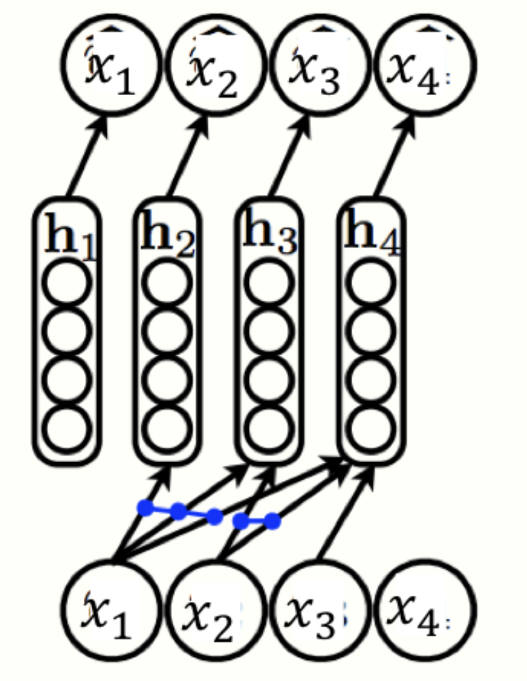

  where $\theta={W\in \mathbb{R}^{d\times n}, \mathbf{c} \in \mathbb{R}^d, {\boldsymbol{\alpha}^{(i)}\in \mathbb{R}^d}^n_{i=1}, {b_i \in \mathbb{R}}^n_{i=1}}$:

  set of params. for $f_1(.),…,f_n(.)$

  The weight matrix $W$ and bias vector $c$ are shared across the model.

  #num. of params. = $O(nd)$

  Fewer than $O(n^2d)$(the above model)

  Performance still better than FVSBN !

Learning and Inference

Learning

Recall we want to minimize the following objective :

\[\min_{\theta \in M}d(p_{data},p_{\theta})\]

One common choice for d is KL divergence - the metric to compare 2 distributions.

\[\min_{\theta\in M}d_{KL} (p_{\mathrm{data}}, p_{\theta}) = \min_{\theta \in M }\mathbb{E}_{\mathbf{x} \sim p_{\mathrm{data}} }\left[\log p_{\mathrm{data}}(\mathbf{x}) - \log p_{\theta}(\mathbf{x})\right]\]

Because $p_{data}$ does not contain $\theta$. It is equivalent to find :

\[\max_{\theta \in M} \mathbb{E}_{\mathbf{x} \sim p_{\mathrm{data}} }\left[ \log p_{\theta}(\mathbf{x})\right]\]

Here, $\log p_{\theta}(x)$ refers as the log-likelihood of datapoint x w.r.t the model distribution $p_{\theta}$.

Using Monte Carlo estimation with assumption of i.i.d sampling in dataset $D$, the objective is approximate to:

\[\max_{\theta\in M}\frac{1}{\vert D \vert} \sum_{\mathbf{x} \in\mathcal{D} }\log p_{\theta}(\mathbf{x}) = \mathcal{L}(\theta \vert \mathcal{D}).\]

In implementation, we optimize the objective using mini-batch gradient ascent. Divide the dataset $D$ into batches . The params. can be updated via the following rule:

\[\theta^{(t+1)} = \theta^{(t)} + r_t \nabla_\theta\mathcal{L}(\theta^{(t)} \vert \mathcal{B}_t)\]

$\mathcal{B}_t$: batch dataset at iter. $t$

$r_t$: learning rate at iter. t

Sampling

This is a sequent procedure: first sample $x_1$, then sample $x_2$ conditioned on $x_1$, then sample $x_3$ conditioned on $x_1,x_2$ etc…

For applications requiring real-time generation (such as music generate based on user voice) the sequential sampling might be very expensive.

---